AI Defect Detection: A Practical Guide to Deployment

A 99% accuracy score can still leave a factory exposed when the defective parts are rare, the lighting changes, and the line keeps moving. That's the tension in AI defect detection. The hard part isn't getting a model to look smart in a demo, it's making it reliable when a missed defect means scrap, rework, customer complaints, or a line stop.

Table of Contents

• What AI Defect Detection Really Solves on a Production Line
• The Three Main Types of AI Defect Detection
• Data Requirements and Labeling Strategies
  • Supervised, self-supervised, synthetic, and few-shot
• Model Architectures and the Trade-offs That Matter
• Evaluation Metrics and Benchmarking Beyond Accuracy
  • What to ask for instead
• Deployment, Monitoring, and the Operational Cost of False Alarms
  • What to monitor after go-live
• Verified Real-World Case Studies
• Building the Business Case Without Hiding the Gaps

What AI Defect Detection Really Solves on a Production Line

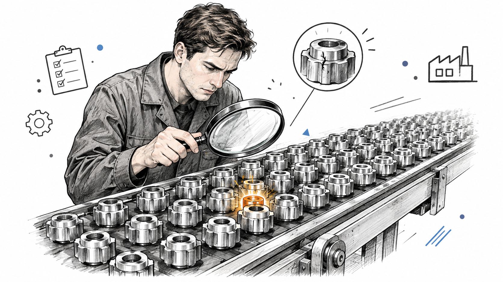
AI defect detection turns inspection into a repeatable production control, but its value depends on more than a classification score. The system must identify rare events while cameras shift, parts vary, surfaces collect dirt, and operators adjust the process. A peer-reviewed review describes the move from conventional image processing to deep-learning machine vision, with controlled studies reporting precision as high as 99.00% and single-image recognition time of 0.12 milliseconds (PMC review).

Those figures describe a test setup, not automatically your line. On a stamping line running 1,200 parts per hour with 0.3% scrap, a model that reports 99% accuracy can still miss 3 to 4 bad parts per shift if recall at the selected threshold is 82%. The missed parts become scrap, rework, or customer returns. False alarms create a different bill: operators stop the line, inspect good parts, and may begin ignoring alerts.

The right production question is therefore specific: will the system catch the defects that matter, using your cameras and process settings, while keeping false alarms within the team's capacity?

Practical rule: set the threshold, latency target, and escalation path against the cost of a missed defect and the cost of stopping for a false alarm.

The system can flag visible flaws before parts leave the line, locate the affected area, and give engineers evidence for root-cause analysis. Validation must connect those outputs to scrap, rework, and line-stop decisions. For a broader explanation of how quality teams apply this technology, see AI for quality control.

The Three Main Types of AI Defect Detection

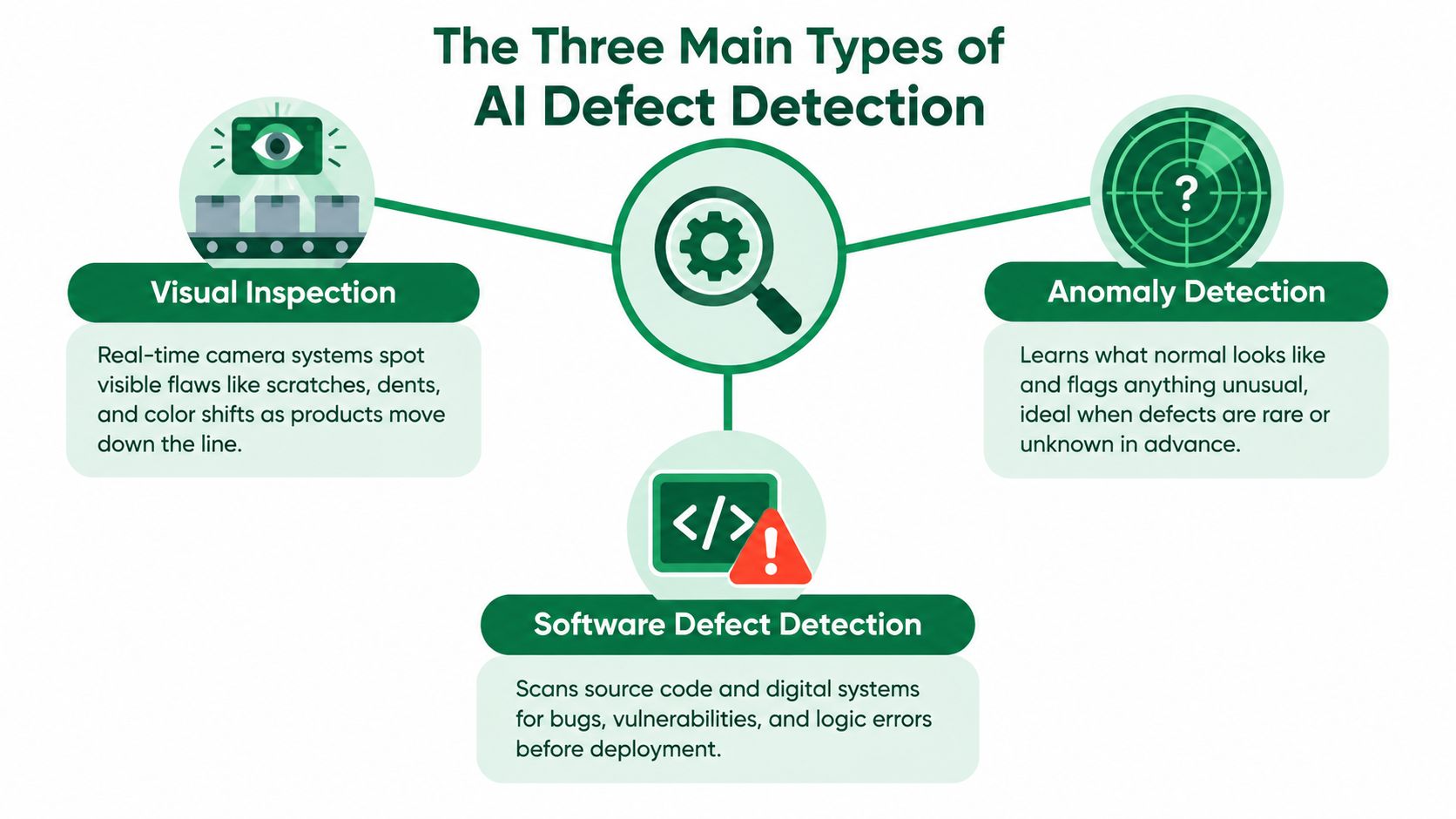
The first type is visual inspection. It analyzes production-line images for scratches, dents, missing components, color shifts, and other visible flaws. Manufacturing systems often begin with classification, which determines whether a defect exists. They may then use localization to identify its position or segmentation to outline its exact shape and area.

The second type is anomaly detection. Anomaly detection models normal images and flags deviations without pre-defined defect classes. This approach suits rare, poorly labeled, or newly emerging defects. It can widen coverage, but unusual does not always mean unacceptable. A lighting change, material variation, or camera shift may trigger an alert that still requires human review.

The MVTec AD benchmark contains 5,354 high-resolution images across 15 object and texture categories. PatchCore reached image-level AUROC as high as 99.6% when trained only on defect-free images (MVTec AD). That result demonstrates benchmark capability, not guaranteed line performance. In production, false alarms consume inspection time and can lead operators to disregard genuine warnings.

The third type is software defect detection. Software defect detection scans source code or digital systems for bugs, vulnerabilities, and logic errors before deployment. It belongs to the wider defect-detection field, but its inputs, failure modes, and response process differ from physical inspection on a factory line.

Choose the type based on the failure mode, not the fashion. A plant with known surface defects needs a different setup from one where new anomalies appear before the team can label them.

The three approaches also differ in output detail. Classification answers whether a defect exists. Localization identifies where it appears. Segmentation traces its boundary at pixel level. Finer-grained output can support repair or root-cause work, but it usually requires more annotation effort and creates more ways for model errors to affect production decisions. The right choice depends on whether the operator needs a reject signal, a defect position, or a measurable shape.

Data Requirements and Labeling Strategies

The steel-surface study is a clear reminder that data scarcity is not a side issue, it shapes the whole inspection problem. That 2024 dataset had 1,104 images, and only 394 showed pitting damage (steel-surface inspection study). Many factories face the same imbalance, where good parts are easy to collect and true defects are rare.

Supervised, self-supervised, synthetic, and few-shot

Supervised labeling is the most direct path. Quality experts mark defects, engineers train a model, and the team works from a shared ground truth. It also consumes the most human time, and inconsistent labels can weaken the signal before training starts.

Self-supervised methods lower the label burden by learning structure from unlabeled images first. They fit plants with lots of image data and very few defect examples. Synthetic defect generation helps when real defects are too scarce to collect quickly, but generated variety can drift from what occurs on the line. Few-shot learning sits between the two, useful when the team has only a small number of real examples but still needs the model to adapt.

The budget often goes to labeling discipline, not architecture choice. If the domain expert and annotator disagree on what counts as a defect, the model inherits that confusion.

A practical workflow starts with a narrow defect definition. Define pitting as dark pits larger than 0.5 mm on brushed steel, have two annotators label 200 images in CVAT, then settle disagreements with the quality engineer before freezing the label guide. That kind of example keeps the team aligned on what is in scope and what is not.

For the inspection record itself, standardize the fields you will need later for traceability and audit. If you need a reference for the data structure, the compare first article data fields page is a useful starting point because it ties the record to the decision the plant needs to make.

Strategy	Typical data need	Strength	Best fit
Supervised	Many labeled defect examples	Clear defect classes	Stable products with known defect types
Self-supervised	Many unlabeled images, few labels	Lower labeling burden	Rare defects or slow label creation
Synthetic	Real images plus generated variants	Faster coverage of edge cases	Early prototyping and hard-to-capture flaws
Few-shot	Very few labeled defects	Fast adaptation	New products or scarce defects

Model Architectures and the Trade-offs That Matter

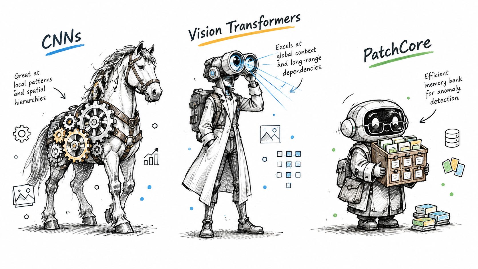
Three architecture families appear repeatedly in industrial inspection. CNNs are the workhorse because they learn local patterns efficiently, supporting the shift from hand-engineered vision features to representations learned directly from images. Vision Transformers model relationships across wider parts of an image, which can help when a defect depends on surrounding structure. Feature-memory methods such as PatchCore take a different route, comparing new image patches with examples of normal production.

The newest model is not automatically the best choice. A survey of more than 50 machine-learning vision systems across automotive, aerospace, assembly, and general manufacturing found that gains depended heavily on dataset fit and integration effort, while 77% of implementations remained at prototype or pilot scale (survey).

A model that wins on paper can still lose on the line if it is slow, brittle, or difficult to integrate.

Start architecture selection with production constraints. A short inspection window makes latency as important as recall. Frequent product changes increase the value of a simple update path and manageable retraining. A rare defect may favor anomaly detection, while clearly labeled defect classes may suit a supervised CNN. The AI image recognition guide offers useful context on how image inputs shape recognition systems.

Specify the operating conditions before comparing models: lock exposure at 2ms, use diffuse dome lighting at 5500K, and require GigE Vision output compatible with the plant's PLC or MES. Then measure recall, inference time, review workload, and false rejects on representative production images. A small benchmark gain is not worthwhile if it creates rework, scrap, or line stops.

Evaluation Metrics and Benchmarking Beyond Accuracy

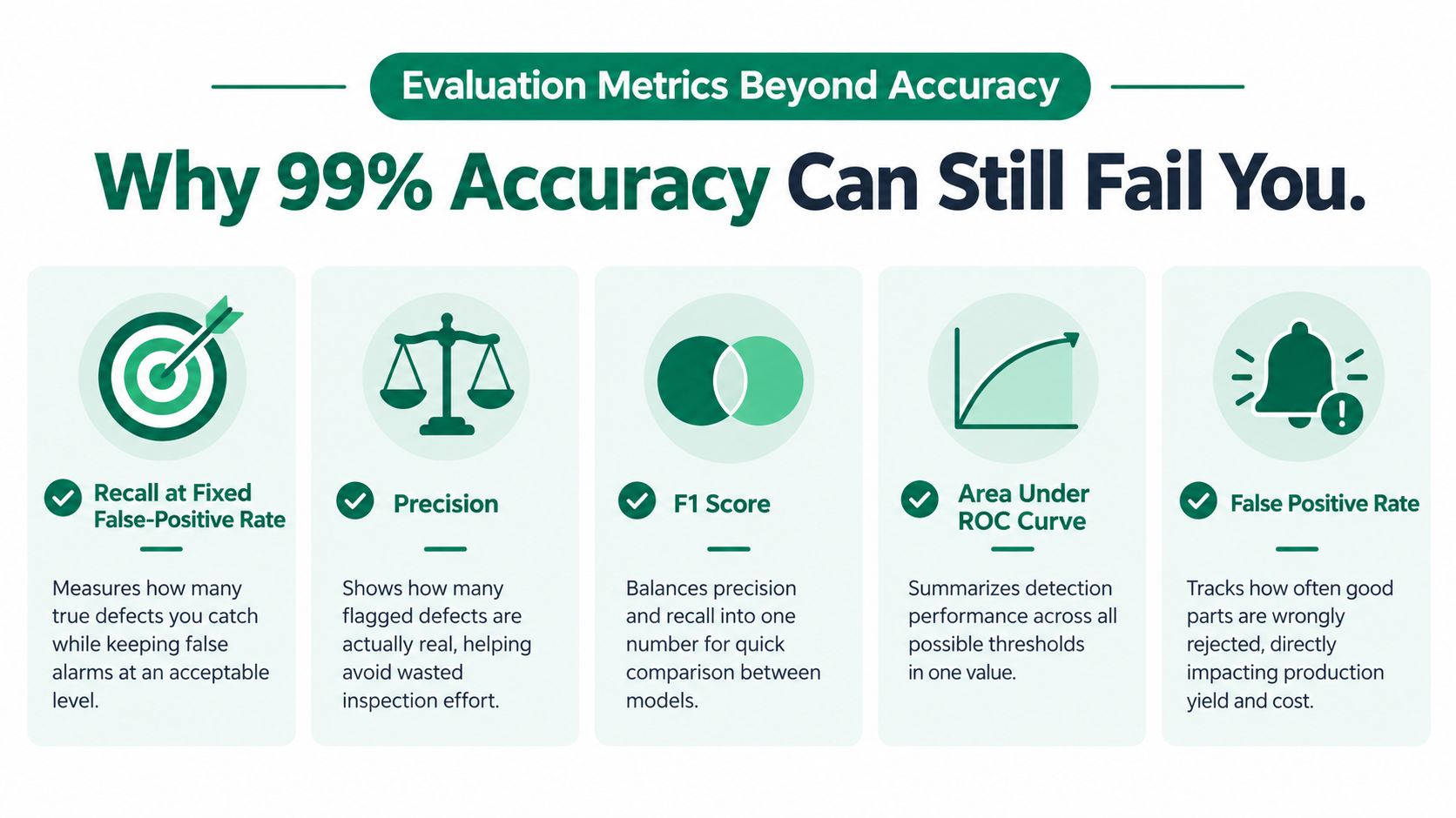
The wrong way to evaluate AI defect detection is to lead with accuracy and stop there. Accuracy can look excellent in a class-imbalanced setting and still hide the fact that the model misses too many bad parts or rejects too many good ones. That's why the operating point matters, not just the headline score.

The Valeo Anomaly Dataset makes that clear. On 5,000 industrial images, EfficientAD reported 89.1% classification AUROC but also a 44.5% false-positive rate at 95% true-positive rate (Valeo Anomaly Dataset). That combination is exactly why a vendor can quote a strong benchmark and still leave operations with an unusable system.

What to ask for instead

A credible evaluation set should include recall at a fixed false-positive rate, because quality teams care about how many defects are caught without overwhelming the line. It should also include precision, because false alarms consume inspection time and erode trust. F1 score helps compare models quickly, though it still hides the underlying cost structure if scrap and warranty costs differ widely.

You also want to separate image-level from defect-level performance. A model can identify that something is wrong without correctly locating the defect. That matters when the downstream action depends on the defect's shape or boundaries. And because class imbalance is the norm, AUROC should never be treated as a production guarantee on its own. It summarizes ranking behavior, not business impact.

A good acceptance test ties the threshold to cost, then checks whether the model survives new lighting, new batches, and new camera positions.

A practical acceptance package should include a confusion matrix weighted by scrap and rework costs, a threshold chosen from production trade-offs, and tests across lighting, materials, camera positions, product variants, and equipment changes. If your data pipeline supports it, add audit samples for borderline cases and review them with operators before release. That's how you keep a benchmark from becoming a false sense of security.

Deployment, Monitoring, and the Operational Cost of False Alarms

A trained model becomes useful only when it survives the line, the operators, and the escalation path. Production setup starts with practical choices: whether inference runs at the edge or on a server, how alerts enter the PLC, MES, or SCADA, and who owns the threshold when the defect mix changes. Those decisions determine whether a promising benchmark becomes a working inspection system.

False alarms turn model output into operating cost. A production inspection study reported that improving the end-to-end inspection setup reduced the false-error rate from 16.83% to a much lower level. The result shows why cameras, integration, workflows, and review rules matter alongside the model. If good parts are repeatedly flagged, operators spend time checking them, trust falls, and scrap or rework can rise.

What to monitor after go-live

Monitor embedding drift weekly, the false-reject rate for every shift, and the minutes operators spend reviewing alerts. Also track defect prevalence, because a changing base rate alters the meaning of the same threshold. Assign the quality engineer to retune the threshold if false rejects exceed 2% for two consecutive shifts. The production manager should review the trend when manual-review time rises, even if the model's headline accuracy remains unchanged.

Practical rule: if alert volume changes but the confirmed defect rate does not, investigate model drift, threshold settings, or an upstream process change.

Alert quality affects adoption. A stream of noisy notifications trains operators to delay or ignore warnings, much like other monitoring systems. Guidance on how continuous threat modeling reduces alert fatigue reinforces the same operational lesson: fewer, better-supported alerts are more useful than a larger volume of weak signals.

Keep human review for low-confidence cases, refresh the normal reference set after tooling or camera changes, and sample missed-defect cases through an audit loop. Review those findings with quality and operations owners, then record whether each change affects scrap, rework, review time, or line stops. The aim is to improve throughput and decisions, not add another source of noise.

Verified Real-World Case Studies

Production results show why validation must include operating cost, not accuracy alone. In an Intel tire-manufacturing case, cameras, machine learning, and Intel processor-based industrial PCs reportedly delivered 99.9% defect-detection accuracy while inspecting two tires per second. The system reduced labor costs by about $49,000 per production line and cut customer complaints by more than 10,000 annually (Intel case study). At that inspection rate, false rejects would create a large review queue. Keeping them under control is therefore part of the business result, because every unnecessary hold consumes operator time and can delay production. The operational lesson is clear: throughput and false-alarm control helped protect the reported labor saving.

The semiconductor review exposes a different validation gap. Reported accuracy across manufacturing vision systems often reached 98–99%, yet only 17% of reviewed systems were in high-volume manufacturing; 83% remained at prototype or pilot stage (semiconductor review). A benchmark can show that a model recognizes test images. It does not prove that operators can review its alerts, that thresholds remain stable, or that the line can absorb false rejects.

A steel-surface study reported 98.7% recall on real industrial data. Recall measures how many actual defects the system found, making it useful when missed defects carry the highest cost.

A related railway example appears in how Hitachi uses AI to detect railway overhead line defects near real time. Across these cases, deployment evidence matters as much as the model score.

Building the Business Case Without Hiding the Gaps

A credible business case for AI defect detection starts with cost buckets the plant already feels: scrap, rework, warranty exposure, customer complaints, and line interruptions. Then map the model to those outcomes. A classifier with strong benchmark results can still lose money if it sends too many good parts to manual review, slows operators, or needs frequent retuning as products, lighting, or materials shift.

That validation gap is where many ROI stories break. A model can look accurate in testing and still create daily friction on the line. The practical question is not “Does the model find defects?” It is “At the operating threshold we will run, do avoided losses exceed review labor, false rejects, and revalidation work?”

Use measured operating cost, not model optimism. If a false alarm pulls an operator for inspection, add that labor. If a hold delays shipments or creates rework queues, add that too. The monthly value equation is simple: avoided scrap, rework, and warranty cost, minus false-reject review hours times labor rate, minus revalidation cost.

For teams that want more grounded implementation examples, the Applied library is a useful reference because it organizes real deployments by company, use case, tools, and results.